Introduction
A mid-sized company is running its reporting the way it has for years.
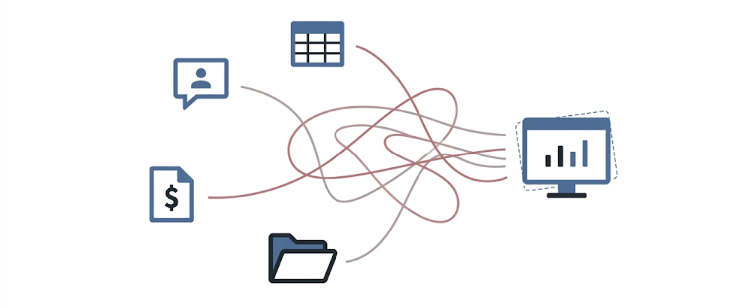
Sales data lives in the CRM. Finance data lives in a separate accounting tool. Operations data sits in spreadsheets that get emailed around and manually merged every Monday. A developer has built a few custom scripts to pull it all together once a week. The BI dashboard on top of it all is only ever as fresh as the last manual refresh.

Someone in leadership reads an article about “the modern data stack” and asks: do we need this?
It’s a fair question. It’s also one that gets answered badly more often than not, usually by a vendor with something to sell.
The stakes of getting it right are real. As reported by DataStackHub’s 2025–2026 BI statistics analysis, organisations with mature, BI-driven strategies achieve an average ROI of 127% within three years of deployment and make decisions roughly 2.5x faster than organisations without that maturity. That’s the upside case. It’s also exactly what gets oversold to companies that haven’t yet diagnosed what they actually need.
“Modern data stack” has become one of the most overused, least precisely defined terms in enterprise technology. It gets used to describe everything from a complete cloud-native architecture to a single new BI tool bolted onto an old system. The term has outpaced any shared understanding of what it actually means.
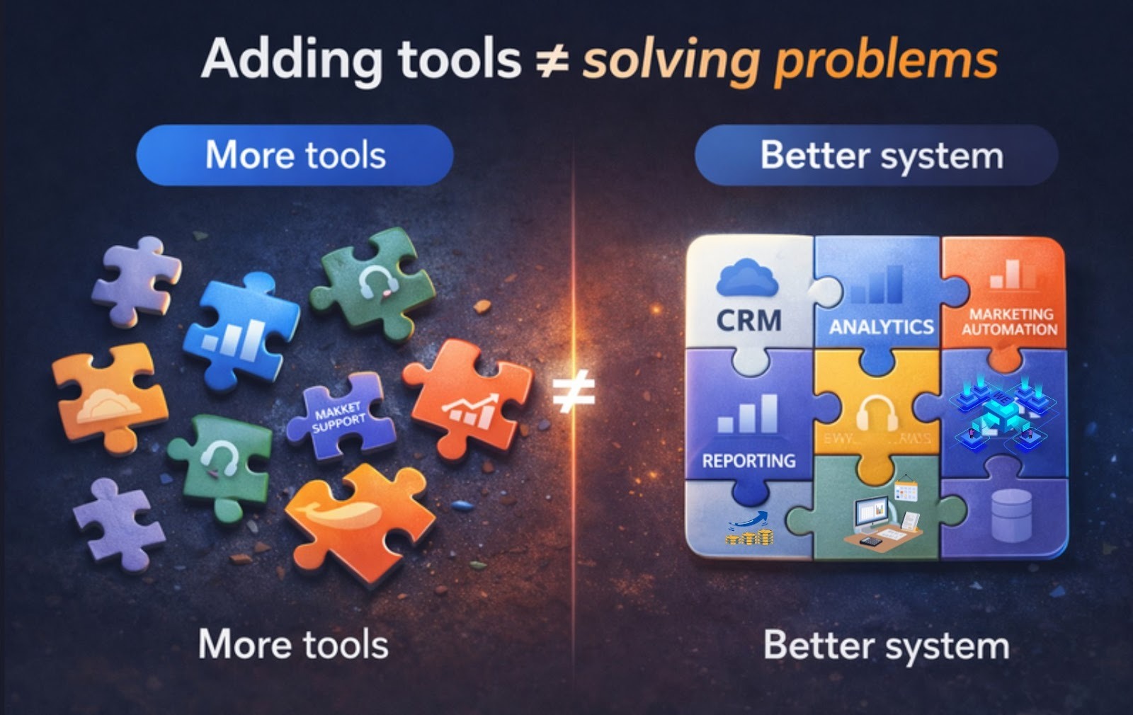
And here’s what gets lost in the noise: most companies asking whether they need a modern data stack don’t actually need the full version of what’s being sold to them. Some need a piece of it. Some need to fix a process problem that no new architecture will solve. A few genuinely need the whole thing.
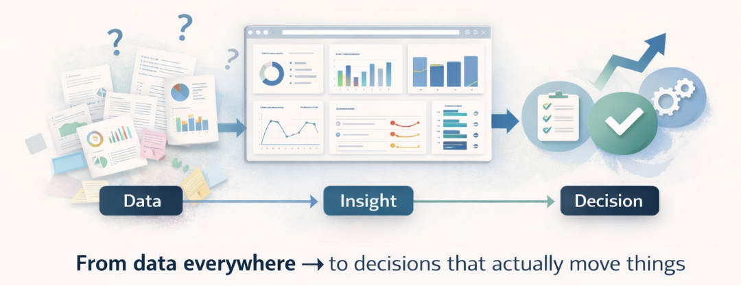
The real question isn’t “what is a modern data stack.” It’s “what problem would this actually solve for us, specifically, and is that the problem we have?”
This article answers both.
What Is a Modern Data Stack, Actually
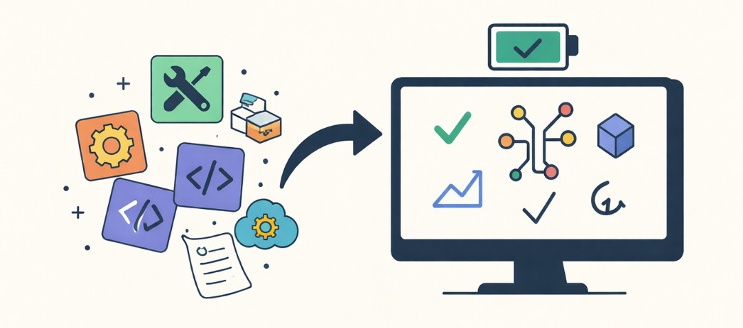
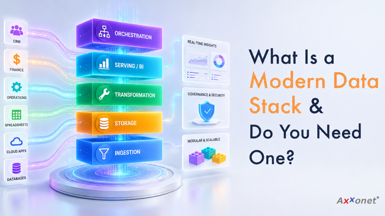
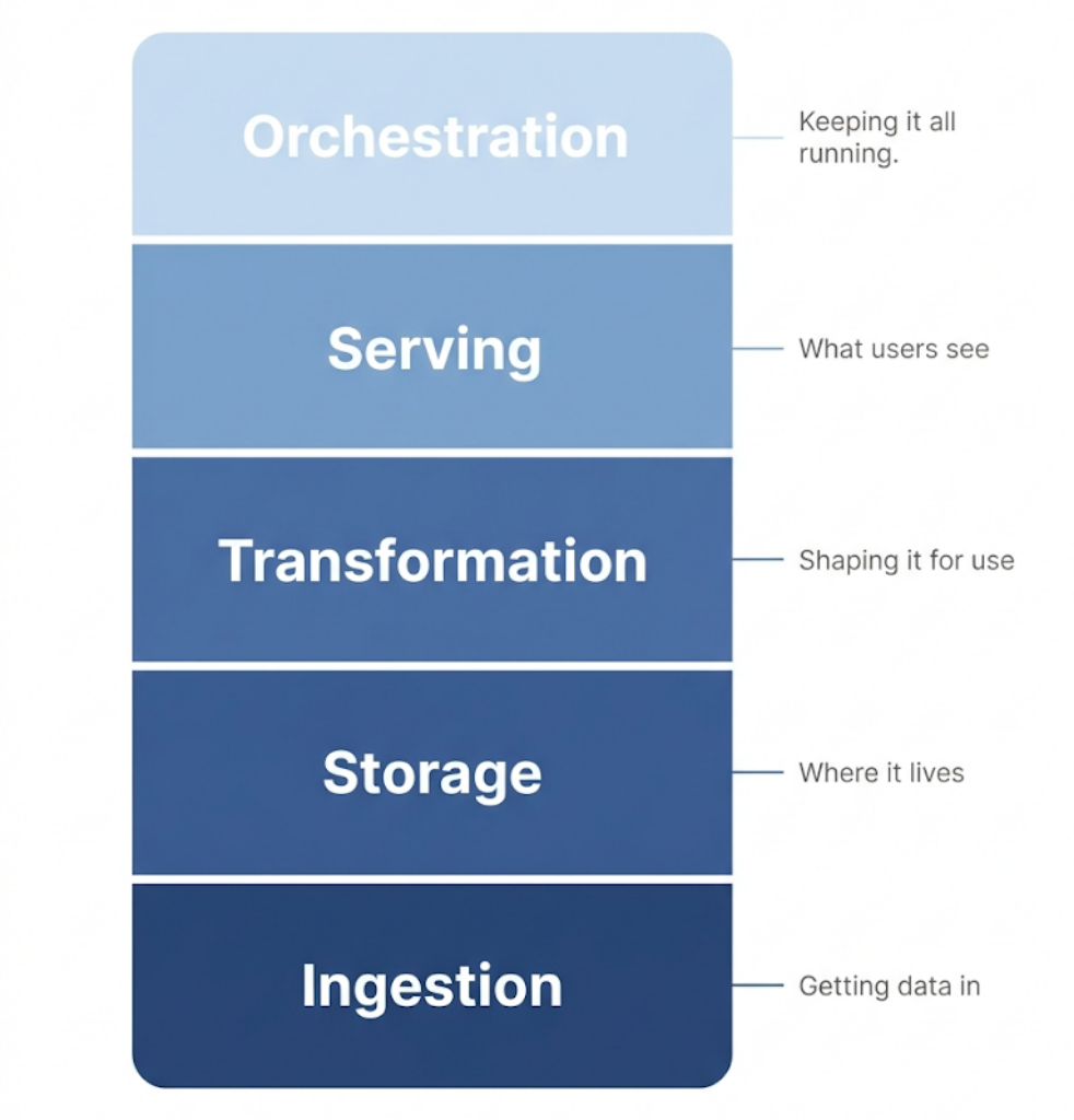
Stripped of the buzzwords, a modern data stack is a modular, cloud-native set of tools that handle data as it moves through four stages: getting it in, storing it, transforming it, and putting it in front of the people who need it.
That’s the whole idea. The “modern” part isn’t about being new for its own sake. It’s about being modular and decoupled; each piece of the stack can be replaced or upgraded independently, rather than being locked into one vendor’s all-in-one platform.
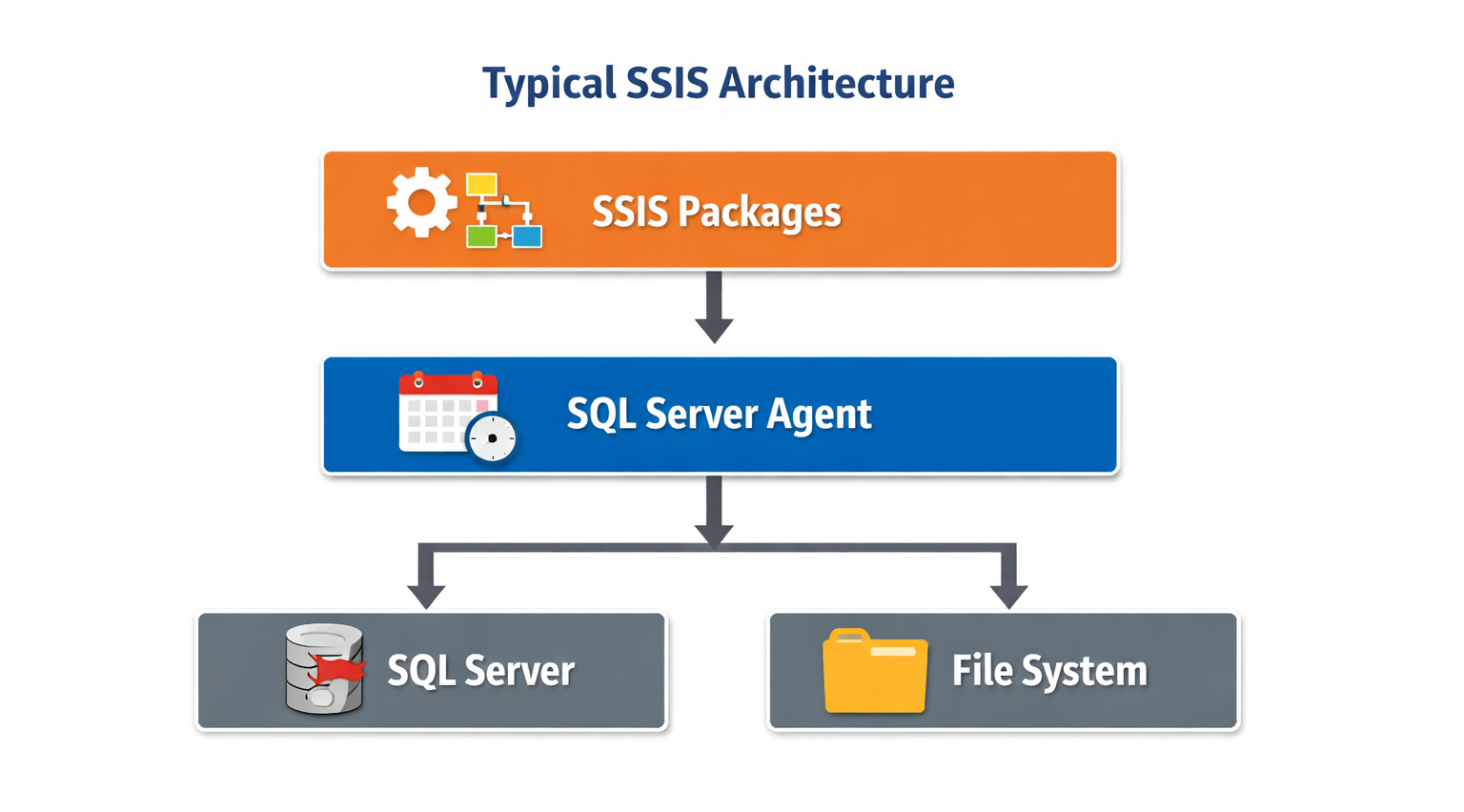
Compare that to the traditional model: a single vendor’s data warehouse, tightly bundled with its own ETL tools and reporting layer, where changing any one piece usually means a painful migration of the whole system.
The modern approach unbundles that. Ingestion is its own layer. Storage is its own layer. Transformation is its own layer. Reporting and analytics sit on top, often pulling from multiple sources at once. Each layer can be swapped out as needs change, without tearing down everything else.
A global benchmark survey of 500 senior data and technology leaders, conducted by Fivetran in late 2025, found that 73% of enterprise data initiatives fall short of expectations despite average annual data budgets exceeding $29 million, and that nearly 62% of organisations still describe their own data maturity as low. The gap isn’t investment. It’s architecture. The pace of adoption is real. So is the confusion about what’s actually being adopted.
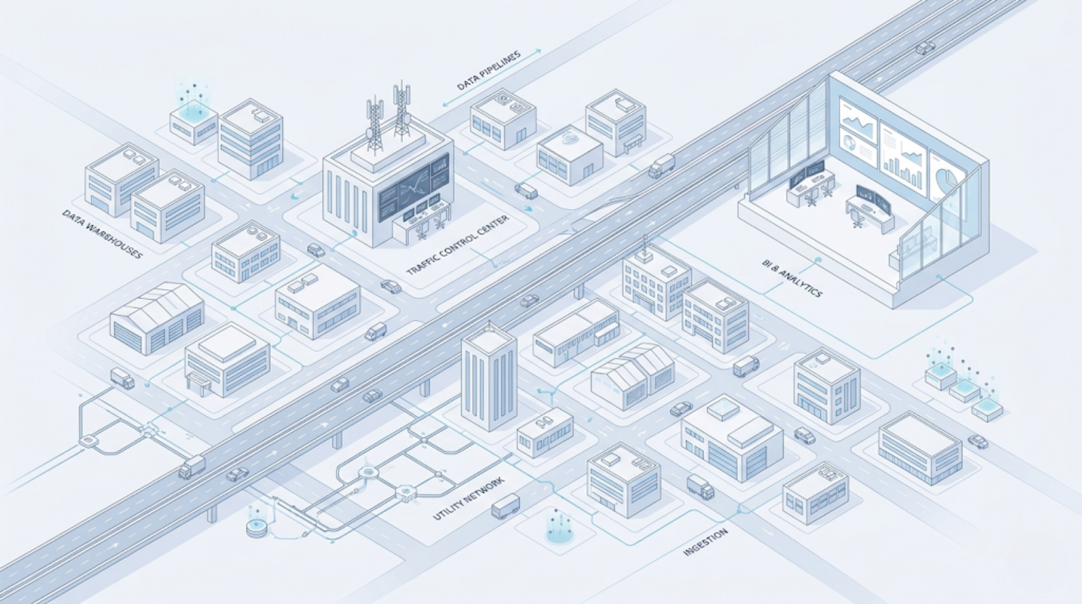
The Layers of a Modern Data Stack
Here’s what the stack actually looks like, layer by layer.
Ingestion and Integration
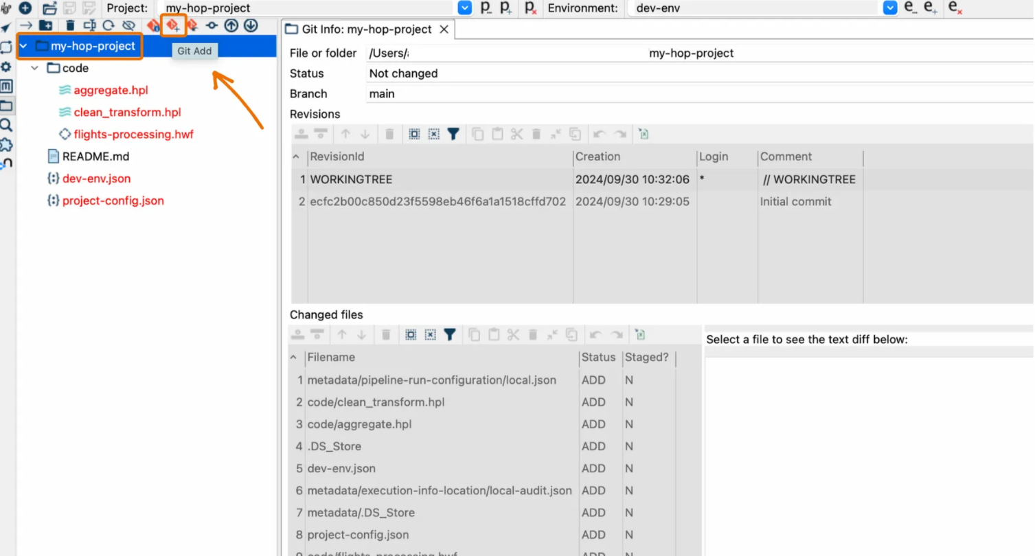
This is how data gets from where it’s created into the stack. It includes batch-based extraction tools, API-based connectors, and increasingly, Change Data Capture (CDC), which captures changes in source systems in near real time rather than waiting for scheduled batch jobs.
This layer ranges from open-source orchestration frameworks to fully managed connector platforms, depending on the complexity and volume of sources involved. For organisations dealing with high-frequency transactional data, CDC pipelines are increasingly the standard; we covered this in detail in Change Data Capture with Debezium, Kafka & Apache Hop.
Ingestion is also where most data quality problems actually originate, not downstream in storage or reporting. AVIA’s piece on the gap between the site data you think you have and the data you actually have is a good illustration of this from the field-operations side: inaccurate data captured at the source creates downstream cost no amount of clever transformation logic can fully fix.
Storage
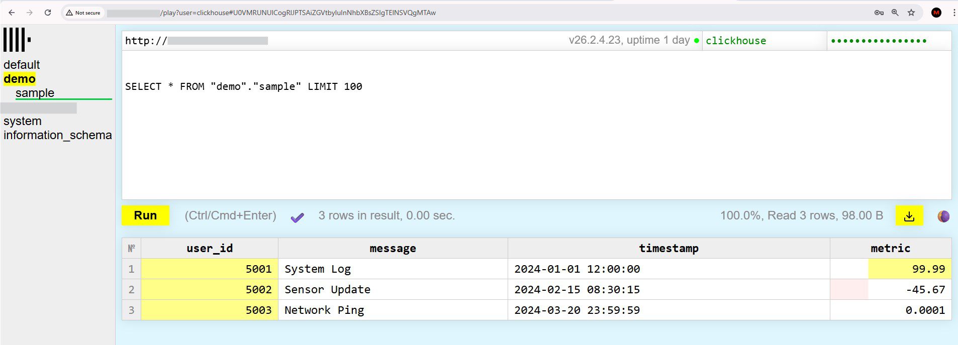
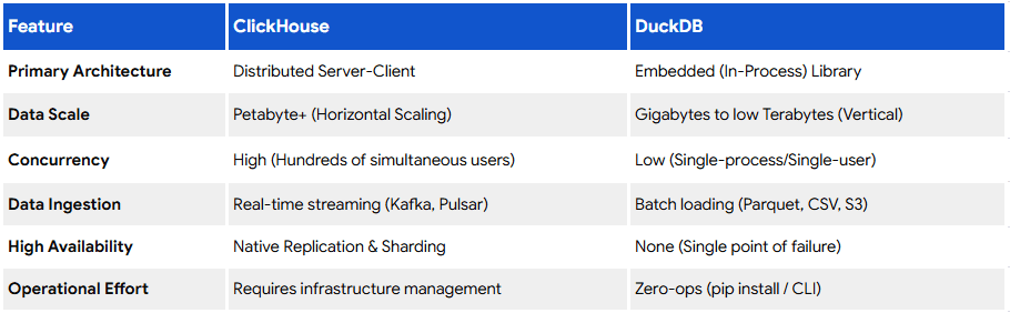
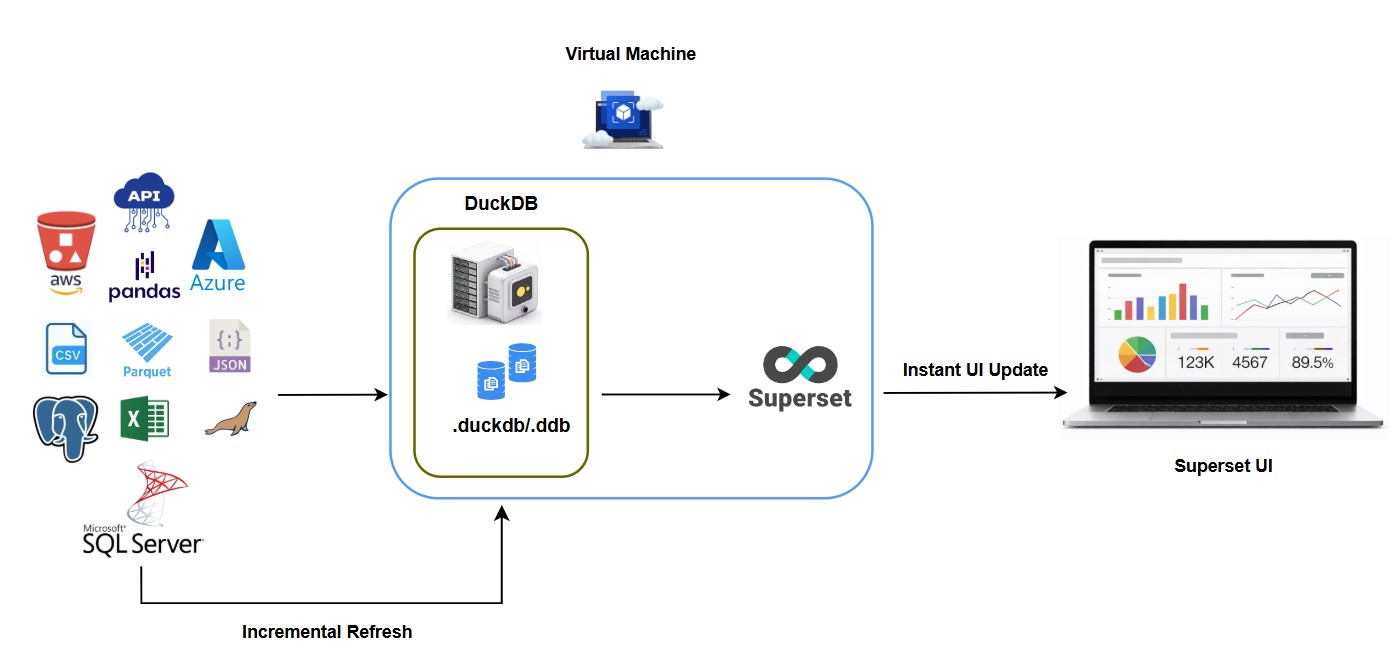
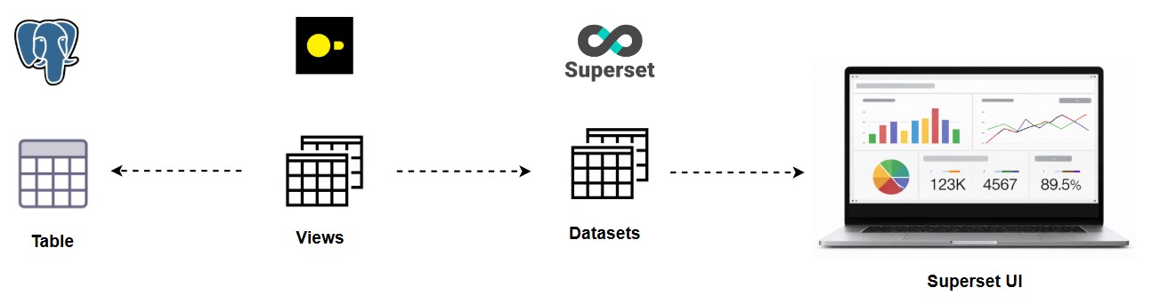
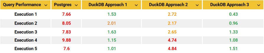
Once data is flowing in, it needs somewhere to live. Large-scale cloud data warehouses and lakehouse architectures dominate this layer at enterprise scale. But not every organisation needs that scale. Lighter analytical engines have become a serious option for mid-sized workloads that don’t justify the cost or complexity of a full warehouse, something we explored in DuckDB for Enterprise Analytics and in our comparison of DuckDB and ClickHouse for cost-conscious analytics. Choosing the right tier here, rather than defaulting to the largest available option, is one of the more consequential decisions in the entire stack.
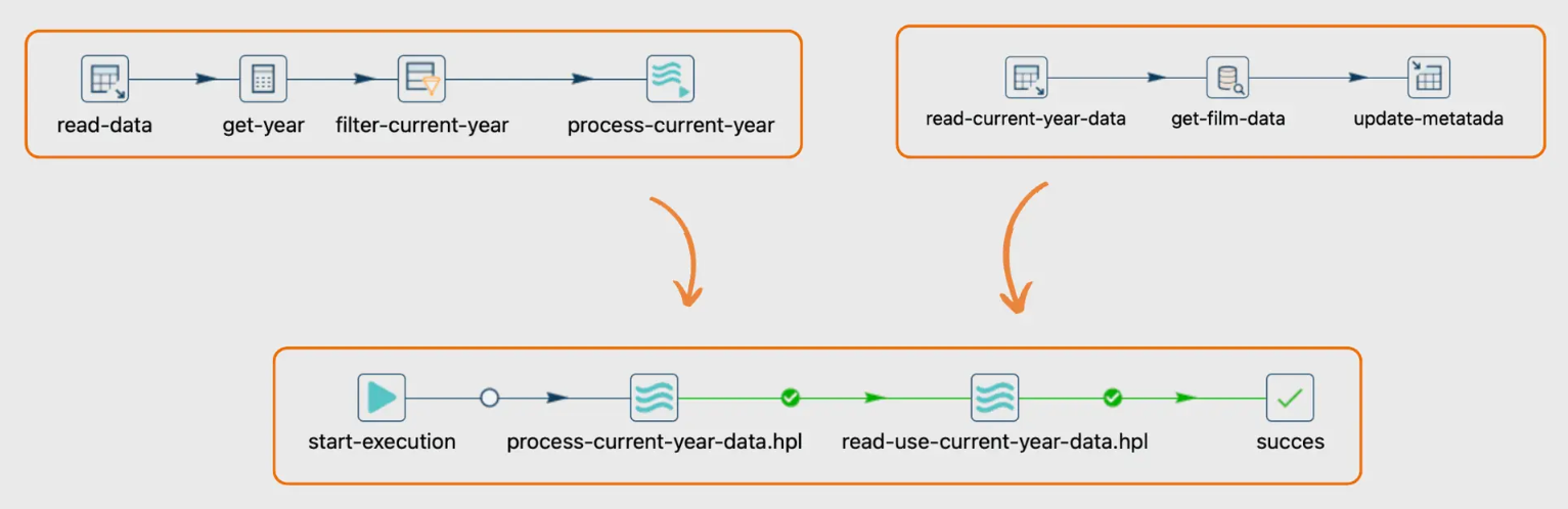
Transformation
Raw data rarely arrives in a shape that’s useful for reporting. This layer cleans, joins, and models data into structures that make sense for analysis, typically using SQL-based transformation logic, orchestrated through a dedicated workflow engine that manages dependencies and run order.Raw data rarely arrives in a shape that’s useful for reporting. This layer cleans, joins, and models data into structures that make sense for analysis, typically using SQL-based transformation logic, orchestrated through a dedicated workflow engine that manages dependencies and run order.Raw data rarely arrives in a shape that’s useful for reporting. This layer cleans, joins, and models data into structures that make sense for analysis, typically using SQL-based transformation logic, orchestrated through a dedicated workflow engine that manages dependencies and run order.
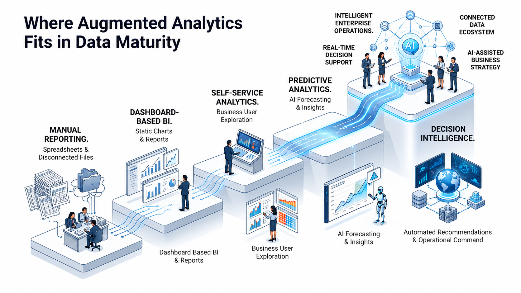
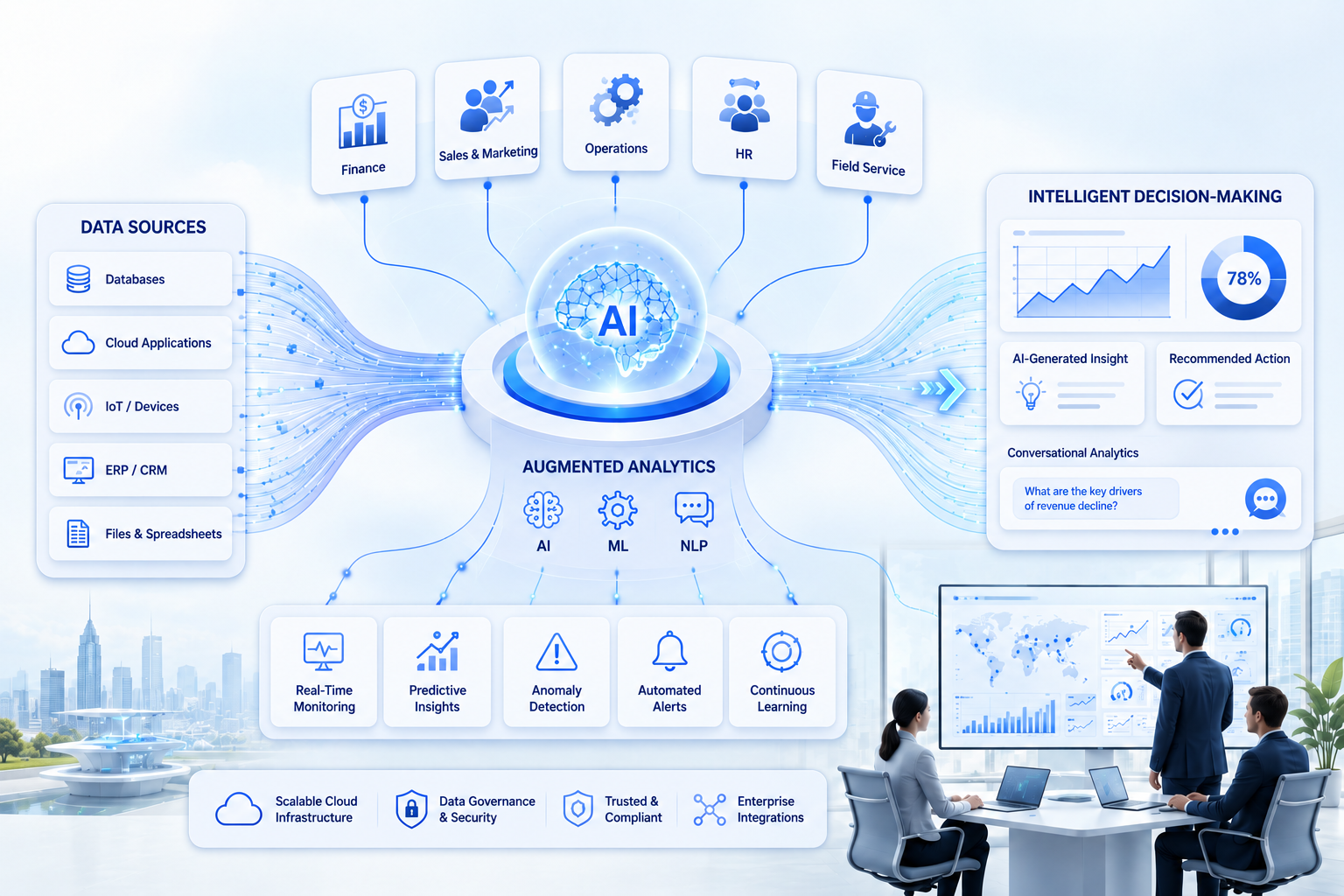
Serving and BI
This is the layer business users actually see: dashboards, reports, and increasingly, natural-language query interfaces. This is also where augmented analytics capabilities live, surfacing insights automatically rather than requiring every question to be manually built into a report. Axxonet works at this layer extensively as part of our analytics consulting practice, helping organisations build governed, accessible reporting on top of whatever sits underneath it.
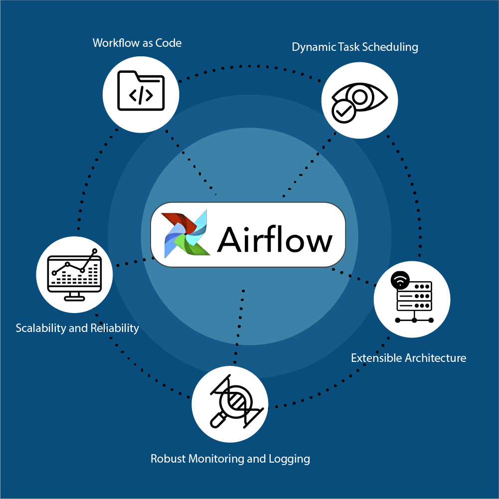
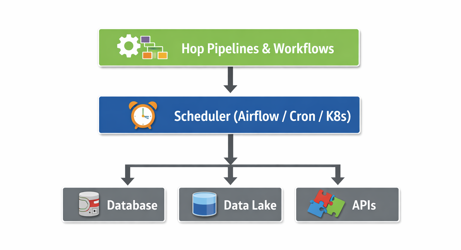
Orchestration and Monitoring
Tying it all together requires scheduling, dependency management, and observability, making sure pipelines run when they should and alerting someone when they don’t. This layer is often integrated with workflow automation platforms; see our work on integrating Apache Hop with n8n for an example of this in practice.
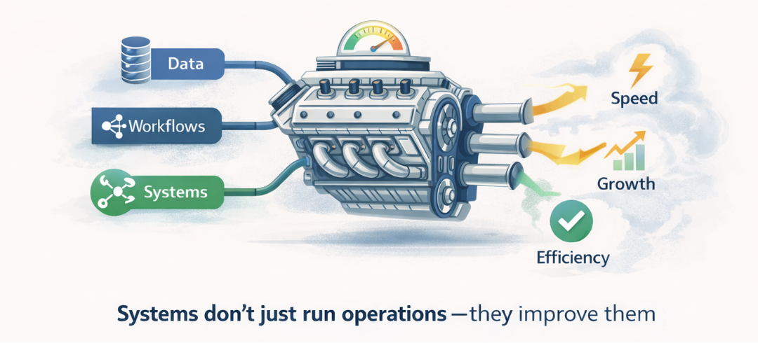
None of these layers exists in isolation. The “stack” is the integration between them, which is also where most of the real engineering effort goes.
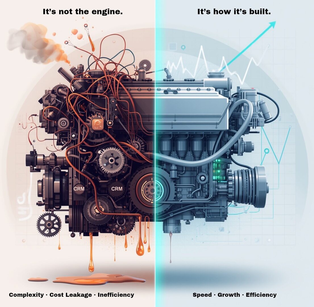
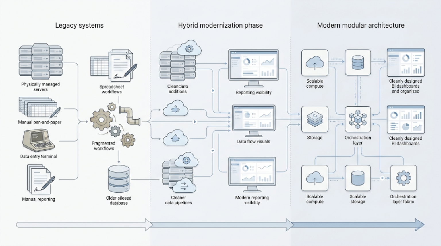
How This Differs From the Traditional Data Warehouse Model
The shift from traditional to modern isn’t just a technology upgrade. It’s a different operating model.
The traditional approach was monolithic by design. One vendor provided the database, the ETL tooling, and often the reporting layer too, bundled together, sold as a single platform. That had real advantages: one throat to choke, one system to learn, predictable support. It also had real costs: vendor lock-in, slow time-to-change, and infrastructure that was expensive to scale because compute and storage were bundled together rather than priced independently.
The modern approach decouples storage from compute, separates ingestion from transformation, and lets you pay for what you actually use rather than provisioning for peak capacity year-round. It’s built for cloud-native scaling and increasingly for near-real-time data rather than overnight batch jobs.
Traditional Warehouse | Modern Data Stack | |
Architecture | Monolithic, single-vendor | Modular, best-of-breed |
Scaling | Provisioned capacity | Usage-based, elastic |
Time to Change | Slow, often requires migration | Fast, layers swap independently |
Data Freshness | Typically batch, overnight | Near real-time capable |
Cost Model | Fixed infrastructure cost | Variable, usage-based |
Vendor Relationship | Single vendor, deep lock-in | Multiple vendors, more flexibility |
The case for getting this right is more than architectural preference. According to Integrate.io’s analysis of enterprise integration benchmarks, organisations with strong system integration achieve 10.3x ROI from their data and AI initiatives, compared to just 3.7x for organisations with poor connectivity between systems. The difference isn’t the tools themselves; it’s whether those tools are actually talking to each other.
The important nuance that gets lost in most “modern data stack” pitches: modern doesn’t automatically mean better for your situation. A well-run traditional warehouse, sized correctly for genuinely batch-oriented reporting needs, can still be the right tool. The question is whether your actual requirements have outgrown it, not whether it’s old.
Do You Actually Need One?
This is the question that matters. Here’s how to answer it honestly.
Signals that point toward a modern data stack:
- You’re manually stitching together data from five or more sources, and that process eats real time every week.
- Reports take days to produce because the data feeding them is scattered, duplicated, or requires manual reconciliation.
- You’re paying for warehouse compute capacity you don’t use most of the time, or regularly hitting capacity limits during peak periods.
- Your business decisions increasingly depend on near-real-time data, and your current batch-based setup can’t deliver it.
- Every new data source requires custom engineering work before it can be reported on.
- Your BI tool is sitting idle, bottlenecked by slow upstream ETL processes that take hours or days to run.
Signals that suggest you don't need the full stack yet, and that's a legitimate answer:
- You have a handful of data sources and a small team, and a lighter setup, sometimes a single well-chosen tool, solves the actual problem without the overhead of a multi-tool architecture
- Your reporting needs are genuinely being met, and the friction you’re feeling is organisational rather than technical, a process problem, not a data architecture problem
- You don’t yet have the in-house data engineering capability to manage and maintain a multi-tool stack, and adding that complexity now would create more operational risk than it removes
Here’s a quick way to sense-check where you land:
Question | If Yes, Lean Toward… |
Are you manually stitching together data from 5+ sources? | Modern stack |
Is your reporting blocked by slow, manual ETL processes? | Modern stack |
Do you have a small team and genuinely simple reporting needs? | Lighter setup, not the full stack |
Do you need near-real-time data to support decisions? | Modern stack |
Is the actual friction organisational rather than technical? | Fix the process first |
Do you lack in-house data engineering capability today? | Build capability before adding complexity |
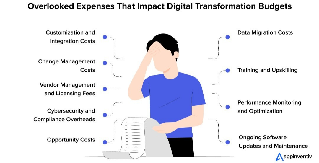
The Hidden Costs of Modernising Too Early
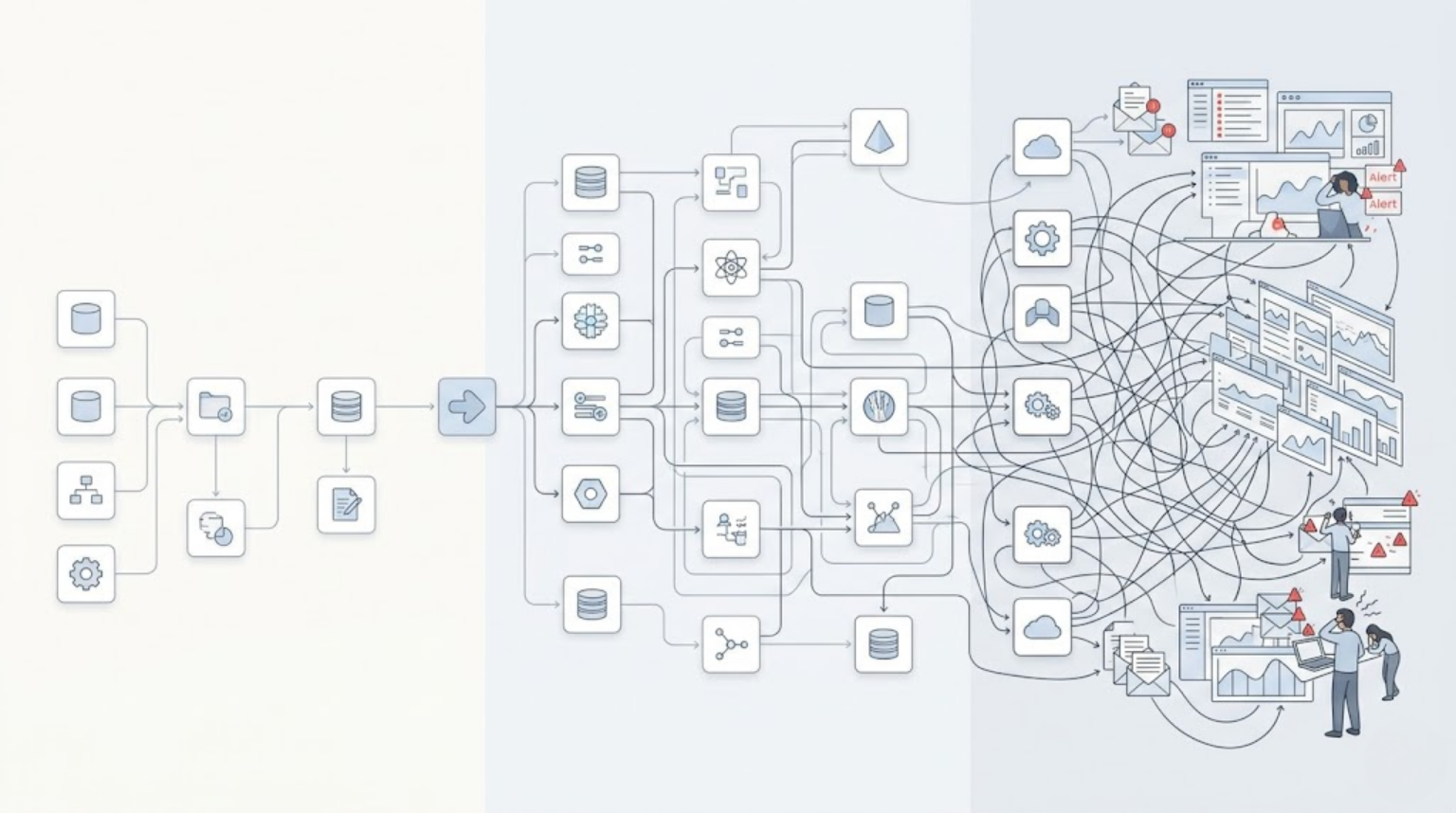
Adopting a modern data stack before you actually need one, or doing it without a clear plan, creates problems that are easy to miss until you’re inside them.
- Tool sprawl. Assembling six different best-of-breed tools sounds appealing in a vendor comparison chart. In practice, tools that don’t integrate cleanly create new manual work, exactly the kind of friction the modern stack was supposed to eliminate. As reported by Integrate.io’s 2026 benchmark study, the average enterprise now runs close to 900 applications, but only around 29% of them are properly integrated with each other, meaning most “modern” environments are already more fragmented than they look from the outside.
- Integration overhead becomes your problem. A monolithic system bundles integration work into the vendor’s responsibility. A modular stack shifts that work to you. Every connection between tools is now something your team owns, monitors, and fixes when it breaks.
- The skills gap is real. Most modern stack tools assume a level of in-house data engineering capability that many mid-sized organisations don’t yet have. Adopting the tooling without that capability just moves the bottleneck, from “we don’t have the data” to “we have the data but nobody can maintain the pipeline.”
- Costs can creep past what they replaced. Usage-based pricing across multiple tools is easy to underestimate. Without active cost governance, a modern stack assembled from several “pay only for what you use” tools can end up costing more than the legacy system it replaced, just less visibly, spread across several invoices instead of one. The upside case only holds when implementation is disciplined: as noted in DataStackHub’s 2025–2026 BI statistics report, organisations with mature BI practices reduce operational costs by 18–22% through better forecasting and efficiency, but that gain comes from disciplined rollout, not from the tooling alone.
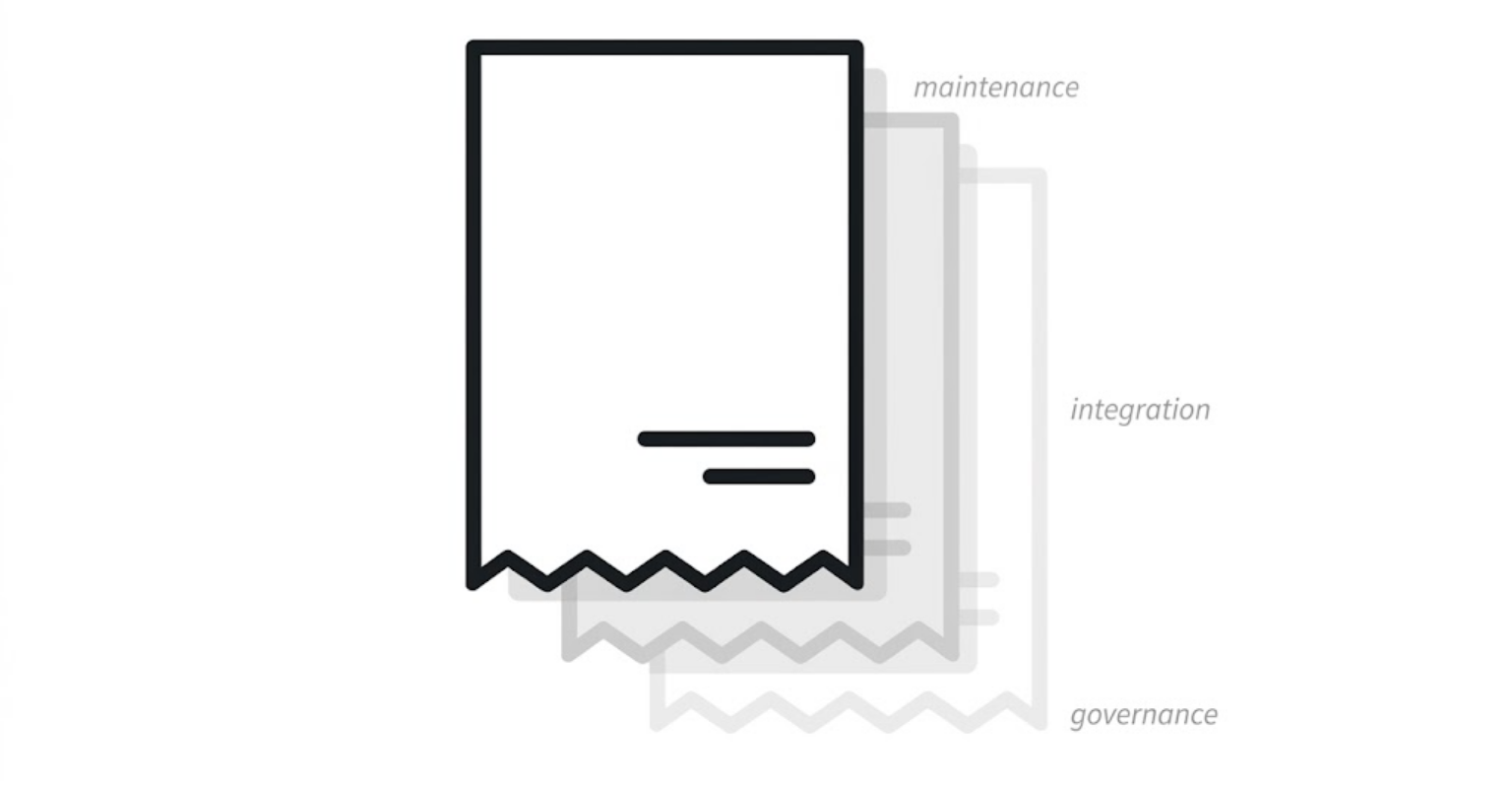
- Governance gaps multiply with each new tool. More systems means more places where data quality can break down, more places where access control needs to be enforced, and more surface area for something to go quietly wrong.
None of this is an argument against modernising. It’s an argument for doing it deliberately.
How to Approach Building One
If the signals point toward a modern data stack, here’s how to build it without falling into the traps above.
- Start with the use case, not the tool list. Define the actual business question or decision this needs to support before evaluating a single vendor. “We need real-time inventory visibility to reduce stockouts” is a use case. “We need a modern data stack” is not.
- Audit what you already have before adding anything. Some of your existing infrastructure may still be the right fit for parts of the problem. Replacing a working component because it’s “legacy” adds cost and risk without adding value.
- Build incrementally, layer by layer. Start with ingestion if that’s the actual bottleneck. Add storage modernisation only if the volume or speed genuinely requires it. Layer transformation and serving on top once the foundation is solid. Trying to stand up every layer simultaneously is where most of the cost and risk concentrates.
- Choose tools that integrate well over tools that are simply popular. A slightly less fashionable tool that connects cleanly with what you already have will outperform a trendier one that requires custom integration work to function.
- Plan governance from day one. Access control, data quality checks, and ownership of each pipeline need to be defined as the stack is built, not retrofitted once something has already gone wrong.
This is the same sequence Axxonet runs before recommending any specific tool: use case first, audit second, incremental build third. It’s a slower start than jumping straight to a vendor shortlist, but it’s the difference between a stack that solves the actual problem and one that just adds more infrastructure to manage.
A Phased Pattern in Practice
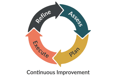
The organisations that modernise successfully tend to do it in layers, not all at once.
A common, practical sequence looks like this: start with Change Data Capture for the data sources where freshness actually matters, moving away from slow batch jobs toward near-real-time ingestion, as we detailed in our CDC implementation work with Debezium, Kafka, and Apache Hop. Pair that with a lighter, cost-conscious analytical engine like DuckDB for workloads that don’t justify a full warehouse, rather than defaulting to the most expensive storage option available. Then layer governed BI on top, once the underlying data is reliable enough to support it.
This is incremental modernisation, solving the actual bottleneck first, adding the next layer only once the previous one is solid, and avoiding the temptation to replace everything at once because a vendor’s reference architecture says so.
Conclusion
A modern data stack is a means, not a goal.
The right question was never “should we adopt one.” It’s “is the pain we’re feeling a data architecture problem actually, and if it is, which layer of it needs solving first?”
Plenty of organisations would get more value from fixing how a single team uses the tools they already have than from assembling a six-vendor modern stack. Others have genuinely outgrown what they’re running and need to modernise in a deliberate, sequenced way. The difference between those two situations is rarely obvious from the outside, and it’s seldom answered correctly by starting with a tool comparison.
Our approach, at Axxonet, is to assess first, build incrementally, and avoid the tool sprawl that turns modernisation into its own ongoing cost. Sometimes that means recommending a single change. Sometimes it means a multi-layer rebuild. The starting point is always the same: understanding what’s actually happening in your data environment today.
Not sure whether your current setup needs modernising or just needs to be used better?
And we'll help you find out.
Frequently Asked Questions
No, though they're related. A lakehouse is a specific storage architecture that combines the flexibility of a data lake with the structure and performance of a data warehouse. It's one possible component of a modern data stack's storage layer, not the entire stack. A modern data stack also includes ingestion, transformation, and serving layers that exist independently of whatever storage architecture sits underneath.
Not necessarily. Many organisations modernise around their existing warehouse rather than replacing it, improving ingestion, adding orchestration, or layering better BI on top, while the core warehouse continues to serve its purpose. Full replacement is only justified when the warehouse itself is the actual bottleneck, usually a question of scale, cost, or architecture fit, not age.
It depends heavily on scope and existing infrastructure. Usage-based pricing across multiple tools makes total cost harder to predict than a single vendor contract, which is exactly why cost governance needs to be built in from the start. A phased approach, solving the most pressing bottleneck first, gives a much clearer cost picture than attempting a full build-out at once.
Mid-sized organisations increasingly manage data volumes and complexity that justify at least parts of a modern stack, but rarely need the full enterprise-scale version. The right approach for a smaller organisation is usually a lighter, more targeted setup: solving the specific bottleneck that's actually causing pain, rather than adopting an architecture designed for a much larger data environment.
ETL (Extract, Transform, Load) transforms data before loading it into storage. ELT (Extract, Load, Transform) loads raw data first and transforms it afterward, inside the warehouse. Most modern data stacks favour ELT, because cloud warehouses can now handle transformation at scale cheaply, and keeping raw data available gives more flexibility for future use cases that haven't been defined yet.
It depends entirely on scope, but a phased build, ingestion first, then storage, then transformation, then serving, typically shows results within the first phase in weeks rather than months. Attempting to build every layer simultaneously extends timelines significantly and is where most of the implementation risk concentrates.
By diagnosing the actual bottleneck before recommending any tool, usually starting with where data quality or speed is breaking down the most, whether that's ingestion, storage, or reporting. The starting layer is different for every organisation, which is why the assessment comes before the architecture, not after.
Axxonet works across both ends of that spectrum. The same diagnostic approach, understand the bottleneck, then build incrementally, applies whether the engagement is a single-layer fix for a smaller team or a multi-layer modernisation for a larger one.
Buying tools before diagnosing the bottleneck. Most failed modernisation efforts start with a vendor shortlist instead of a clear answer to what's actually broken, which usually means the wrong layer gets fixed first, and the real problem is still there once the new tooling is in place.